Comparing to existing features

Highly comparative time-series analysis using hcts
Search…
One of the key goals of highly comparative time-series analysis, is to allow unbiased methodological comparison between the vast literature of time-series analysis tools developed for different applications. By representing features in terms of their outputs across a time-series dataset, the context of a given feature can be assessed by searching the database for features with similar behavior. The search can be done using a diverse range of real and model-generated data, or using a more specific dataset if this is more appropriate for a given application (e.g., looking just at EEG signals). Just like similar time series to a target can be retrieved and visualized, similar features to a given target feature can also be retrieved using TS_SimSearch.
This chapter will give instructions on how you can compare a new time-series analysis feature to our library of over 7000 time-series features using hctsa. We assume that the reader has installed hctsa, which will be required to work with files and compute features.
Setting a data context
The first step is defining the set of features to compare to (here we use the default hctsa library), and the set of time-series data that behavior is going to be assessed on. If you have just developed a new algorithm for time-series analysis and want to see how it performs across a range of interdisciplinary time-series data, then you may want to use a diverse set of time series sampled from across science. This can be easily achieved using our set of 1000 time series, a random selection of 25 such time series are plotted below (only the first 250 samples are plotted to aid visualization):
Pre-computed results for a recent version of hctsa can be downloaded from figshare as HCTSA_Empirical1000.mat.
Alternatively, features can be recomputed using our input file for the time-series dataset, using the input file provided in the same figshare data repository. This ensures implementation consistencies on your local compute architecture; i.e., using TS_Init('INP_Empirical1000.mat'); to initialize, followed by compute commands involving TS_Compute).
However, if you only ever analyze a particular type of data (e.g., rainfall), then perhaps you're more interested in which methods perform similarly on rainfall data. For this case, you can produce your own data context for custom data using properly structured input files as explained here.
EXAMPLE 1: Determining the relationship between a new feature and existing features
We use the (hypothetical) example of a hot new feature, :boom: hot_feature1 :boom:, recently published in Science (and not yet in the hctsa library), and attempt to determine whether it is completely new, or whether there are existing features that exhibit similar performance to it. Think first about the data context (described above), which allows you to understand the behavior of thousands of features on a diverse dataset with which to compare the behavior of our new feature, hot_feature1. This example uses the Empirical1000 data context downloaded as HCTSA_Empirical1000.mat from figshare.
1. Computing the new features
Getting the feature values for the new feature, hot_feature1, could be done directly (using TS_CalculateFeatureVector), but in order to maintain the HCTSA structure, we instead produce a new HCTSA.mat file containing just hot_feature and the same time series. For example, to compare to the HCTSA_Empirical1000.mat file hosted on figshare, you should use the same version of hctsa to enable a valid comparison to the same set of features.
We first generate an input file, INP_hot_master.txt containing the function call, that takes in a time series, x:
1
MyHotFeature(x)     hot_master
Copied!
Any additional arguments to the function MyHotFeature.m should be specified here. MyHotFeature.m must also be in a form that outputs a structure (or a single real number, as explained here).
The interesting field in the structure output produced by MyHotFeature(x) is hotFeature1, which needs to be specified in another input text file, INP_hot_features.txt, for example, as:
1
hot_master.hotFeature1     hot_feature1      hot,science
Copied!
where we have given this feature two keywords: hot and science.
So now we are able to initiate a new hctsa calculation, specifying custom code calls (master) and features to extract from the code call (features), as:
1
TS_Init('INP_1000ts.mat','INP_hot_master.txt','INP_hot_features.txt',true,'HCTSA_hot.mat');
Copied!
This generates a new file, HCTSA_hot.mat, containing information about the 1000 time series, and the new hot feature, hot_feature1, which can then be computed as:
1
TS_Compute(false,[],[],'missing','HCTSA_hot.mat');
Copied!
2. Combining
So now we have both a context of the behavior of a library of >7000 features on 1000 diverse time series, and we also have the behavior of our three hot new features. It is time to combine them and look for inter-relationships!
1
TS_Combine('HCTSA_Empirical1000.mat','HCTSA_hot.mat',true,true,'HCTSA_merged.mat');
Copied!
3. Comparing
Now that we have all of the data in the same HCTSA file, we can compare the behavior of the new feature to the existing library of features. This can be done manually by the researcher, or by using standard hctsa functions; the most relevant is TS_SimSearch. We can find the ID assigned to our new hot_feature in the merged HCTSA file as:
1
load('HCTSA_merged.mat','Operations');
2
Operations(strcmp(Operations.Name,'my_hot_feature'),:)
Copied!
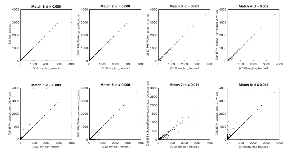
which tells us that the ID of my_hot_feature in HCTSA_merged.mat is 7703. Then we can use TS_SimSearch to explore the relationship of our hot new feature to other features in the hctsa library (in terms of linear, Pearson, correlations):
1
TS_SimSearch(7703,'tsOrOps','ops','whatData','HCTSA_merged.mat','whatPlots',{'scatter','matrix'})
Copied!
We find that our feature is reproducing the behavior of the first zero of the autocorrelation function (the first match: first_zero_ac; see Interpreting Features for more info on how to interpret matching features):
The pairwise distance matrix (distances are 1−∣r∣1-|r|1−∣r∣
, for Pearson correlation coefficients, rrr
) produced by TS_SimSearch provides another visualization of the context of this hot new feature (in this case there are so many highly correlated features, that the matrix doesn't reveal much subtle structure):
4. Interpreting
In this case, the hot new feature wasn't so hot: it was highly (linearly) correlated to many existing features (including the simple zero-crossing of the autocorrelation function, first_zero_ac), even across a highly diverse time-series dataset. However, if you have more luck and come up with a hot new feature that shows distinctive (and useful) performance, then it can be incorporated in the default set of features used by hctsa by adding the necessary master and feature definitions (i.e., the text in INP_hot_master.txt and the text in INP_hot_features.txt) to the library files (INP_mops.txt and INP_ops.txt in the Database directory of hctsa), as explained here. You might even celebrate your success by sharing your new feature with the community, by sending a Pull Request to the hctsa github repository!! :satisfied:
EXAMPLE 2: Determining the relationship between an existing hctsa feature and the rest of the library.
If using a set of 1000 time series, then this is easy because all the data is already computed in HCTSA_Empirical1000.mat on figshare :relaxed:
For example, say we want to find neighbors to the fastdfa algorithm from Max Little's website. This algorithm is already implemented in hctsa in the code SC_fastdfa.m as the feature SC_fastdfa_exponent. We can find the ID of this feature by finding the matching row in the Operations table (ID=750):
1
Operations(strcmp(Operations.Name,'SC_fastdfa_exponent'),:)
Copied!
and then find similar features using TS_SimSearch, e.g., as:
1
TS_SimSearch(750,'tsOrOps','ops','whatData','HCTSA_Empirical1000.mat','whatPlots',{'scatter','matrix','network'})
Copied!
Yielding:
​
 
​
We see that other features in the library indeed have strong relationships to SC_fastdfa_exponent, including some unexpected relationships with the stationarity estimate, StatAvl25.
Combining the network visualization with scatter plots produces the figures in our original paper on the empirical structure of time series and their methods (cf. Sec. 2.4 of the supplementary text), see below:
Specific pairwise relationships can be probed in more detail (visualizing the types of time series that drive any relationship) using TS_Plot2d, e.g., as:
1
theFeatureIDs = [750,544]; % IDs for the two features of interest
2
[TS_DataMat,TimeSeries,Operations] = TS_LoadData('HCTSA_Empirical1000.mat'); % load data
3
featureData = TS_DataMat(:,theFeatureIDs); % take the subset
4
operationNames = Operations.Name(theFeatureIDs); % names of the two features
5
annotateParams = struct('n',6); % annotate six time series with the cursor
6
% Generate an annotated 2-dimensional scatter plot:
7
TS_Plot2d(featureData,TimeSeries,operationNames,{},annotateParams);
Copied!